Hypothesis Testing

Some concepts live in the heart of Statistics and Data Science. Hypothesis testing is one of these concepts. In Inferential Statistics (Inferential statistics makes inferences and predictions about a population based on a sample of data taken from the population in question), there are two ways to make inferences about particular population parameters ( μ : population mean) from sample parameters ( x̅ : sample mean) and to help researchers decide whether the statistical relationship in a sample reflects statistical relationship in population or is just a matter of sampling error.

Firstly we use confidence levels to estimate parameters: “We can be 95% confident that the average GPA (grade point average) of all college students is between 2.7 and 2.9.” We can use hypothesis tests to test and ultimately draw conclusions about the value of a parameter and state, for example: “There is enough statistical evidence to conclude that the mean normal body temperature of adults is lower than 98.6 degrees F.”

In this article, I will explain Hypothesis testing, which may be a difficult concept to grasp at first but I will try to provide an intuitive explanation.

Definition

Hypothesis, in statistics, is a statement about a population where this statement typically is represented by some specific numerical value. Hypothesis testing is an inference method for testing a stated hypothesis. We use a method where we gather data in an effort to obtain evidence about the hypothetical statement.

A hypothesis test evaluates two mutually exclusive statements about a population to determine which statement is best supported by the sample data. These two statements are called the null hypothesis and the alternative hypothesis respectively.

Criminal Trial Analogy

One place where one can consistently see the general idea of hypothesis testing in action is in criminal trials. The criminal justice system (of most countries) assumes that “the defendant is innocent until proven guilty”. In the practice of statistics, we make our initial assumption by stating our two competing hypotheses, the null hypothesis (H0) and the alternative hypothesis (HA), stated as:

• H0: Defendant is not guilty

• HA: Defendant is guilty

In statistics, we always assume the null hypothesis is true. That is, the null hypothesis is always our initial assumption.

The prosecution team then collects pieces of evidence like fingerprints, blood spots, weapons, witnesses, etc, with the hope of presenting **sufficient evidence **to refute the assumption of innocence. (In statistics, data is the ‘evidence’).

The jury then makes a decision based on the available evidence:

• If the jury finds sufficient irrefutable evidence, the jury rejects the null hypothesis and deems the defendant guilty. (We accept that the defendant is guilty and treat him accordingly).

• If there is insufficient evidence, then the jury does not reject the null hypothesis. The jury does not say that the defendant is innocent, just that there is not enough evidence for the conviction. (It’s a different matter that we treat the defendant as an innocent thereafter).

  In statistics, we always make one of two decisions. We either “reject the null hypothesis in favor of the alternate hypothesis” or we “fail to reject the null hypothesis.”

Hypothesis Testing Framework

• Start with a null hypothesis, H0, that represents the status quo.

• Set an alternative hypothesis, HA, that represents the research question, ie that for which we’re testing.

• Conduct a hypothesis test under the assumption that the null hypothesis is true, either via simulation or the theoretical methods (it relies on Central Limit Theorem).

• If the test results suggest that the data do not provide convincing evidence for the alternative hypothesis, stick with the null hypothesis.

• If they do, then reject the null hypothesis in favor of the alternative

In this blog, I will use a case study to further explain hypothesis testing and make a decision using the simulation approach.

Case Study: Gender Discrimination

In 1972, as part of a study on gender discrimination, 48 male bank supervisors were each given the same personnel file and asked to judge whether the person should be promoted to a branch manager job that was described as routine. The files were identical except that half of the supervisors had files showing the person was male while the other half had files showing the person was female. It was randomly determined which supervisors got male applications and which got female applications. Of the 48 files reviewed 35 were promoted. The study is testing whether females are unfairly discriminated against.

Let’s take a look at the data.

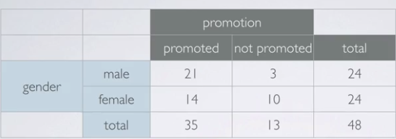
The percentage of males promoted (21 out of 24) is 88%, and the percentage of females promoted (14 out of 24) is 58%. The difference is 30%!

This study shows that there’s a considerable difference (around 30%) in the proportion of males to females promoted. There may be two possible explanations for this result, and these are our two competing claims:

1. There is nothing going on

   The observed difference in proportions is simply due to chance. This is our null hypothesis.

2. There is gender discrimination

That observed difference in proportions is not due to chance, there is discrimination against females. This is the alternative hypothesis.

Now to see which claim is statistically significant, we will simulate the above experiment using a deck of playing cards. Remember, the objective is to conduct a simulation under the assumption that the null hypothesis is true. In other words, assuming there is no gender discrimination, and that the differences in promotion rates noticed are simply due to chance.

There are 52 cards in a deck, however, only 48 files in our experiment. To simulate the experiment, we need to remove some cards to hit a total sample size of 48. The face cards (Jacks, Queens & Kings) represent ‘not promoted’ and the non-face cards (numbers) represent promoted files.

In order for the distribution of face and non-face cards to match the distribution of the promoted and not promoted files, we’re will take out the jokers (extra cards) and three aces and allocate the 1 remaining ace to the face cards so that the total face cards amount to 13 — equal to the total number of ‘not promoted’ files. We’re also going to take out a number card, any number card so that there are exactly 35 number cards left in the deck, representing the promoted files.

Simulation Scheme

1. Face cards: not promoted, non-face cards: promoted;

2. Shuffle the cards, deal into two groups of 24 each, representing males and females.

3. Count how many NUMBER of cards are in each group (representing promoted files).

4. Count the number of Calculate the proportion of promoted files in each group, record the difference (male-female).

In order to obtain a reasonable level of assurance that this simulation is ‘truthful’, the card distribution exercise would have to be carried out many many times, each time the results would be recorded (building up a bank of data) — the more times the cards distribution exercise is carried out, the closer would we be to the ‘truth’ — in other words the confidence level at which we will accept the findings.

Since we’re randomly shuffling the promoted files into two groups and carrying out a card distribution exercise after each shuffle of the cards, we would expect eventually to confirm (or not) that the results of the experiments may be confidently stated as being non-discriminatory towards females. But if the mean distribution differs from the experiment result, then the experiment results may be said to be discriminatory.

Automating the card simulation exercise in R

We would repeat the above card simulation many, many times to build a simulation distribution in order to make a cogent decision. Since manually doing the simulation is time-consuming and there is a chance of errors, I wrote an R script to automate the simulation to obtain the distribution of the differences of promotion rates between males and females.

Here is the R script

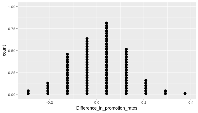
This is what the distribution looks like, called Normal Distribution. The majority of the occurrence of the data is close to 0.0, and most of the occurrence falls within 2 standard deviations (95% confidence level).

So how do we ultimately make a decision?

• If the results from the simulations look like the resultant data of the experiment, then we decide that the difference between the proportions of promoted files, between males and females, was due to chance and that there was no gender bias in the experiment.

• If, on the other hand, the results from the simulations do not look like the data, then we decide that the observed difference in the promotion rates was unlikely to have happened just by chance and that it can be attributed to gender bias. In other words, we conclude that the data provide evidence of a dependency between promotion decisions, and gender-bias or discrimination of females.

Conclusion

From the simulated distribution, it will be noticed that it is rare to get a difference as high as 30%, the calculated difference in the original data. The low likelihood of this event, or a difference even more extreme, suggests that promotion decisions may not be independent of gender, and so we would reject the null hypothesis in favor of the alternate hypothesis.

The probability of observing data, at least as extreme as the one observed in the original study, under the assumption that the null hypothesis is true, is called the p-value. In our case, the p-value is very low as such an extreme outcome is rare.

Our conclusion is then that these data show convincing evidence of an association between gender and promotion decisions made by male bank supervisors.

Wrapping Up

We just walked through a brief example that introduces us to hypothesis tests. In the next blog, I wish to write about the theoretical approach to make decisions between two competing hypotheses.